Starting in XOA v3.2, the gene_panel.json, analysis_summary.html, and transcripts.parquet files will display additional information when Xenium Prime 5K datasets contain pre-designed genes with additional probe sets per gene ("gene boosting"). Learn more about gene boosting in the panel design process on the Xenium Panel Designer website.
The gene_panel.json format is unchanged, however boosted genes will be listed twice: 1) with the 10x Genomics pre-designed gene_coverage and 2) with the boosted gene_coverage and source information.
Below is an example where the original coverage for ACKR3 is 3 probe sets and the boosted coverage is 5 probe sets, for a total of 8 probe sets for this gene:
{
"codewords": [
5226,
6589,
17780
],
"info": {
"gene_coverage": 3
},
"source": {
"category": "base",
"identity": {
"design_id": "hAtlas_v1.1",
"name": "Xenium Human 5K Pan Tissue & Pathways Panel",
"version": "1.1.0"
}
},
"type": {
"data": {
"id": "ENSG00000144476",
"name": "ACKR3"
},
"descriptor": "gene"
}
},
{
"codewords": [
9397,
17171,
4676,
2240,
11249
],
"info": {
"gene_coverage": 5
},
"source": {
"category": "current",
"identity": {
"design_id": "XXXXXX",
"name": "hMulti_100g",
"version": "1.0.0"
}
},
"type": {
"data": {
"id": "ENSG00000144476",
"name": "ACKR3"
},
"descriptor": "gene"
}
}
The analysis_summary.html file provides information about boosted genes on the Summary, Decoding, and Cell segmentation tabs.
On the Summary tab, the Panel Specification table provides the number of boosted genes as part of "Total custom targets (RNA)" metric.
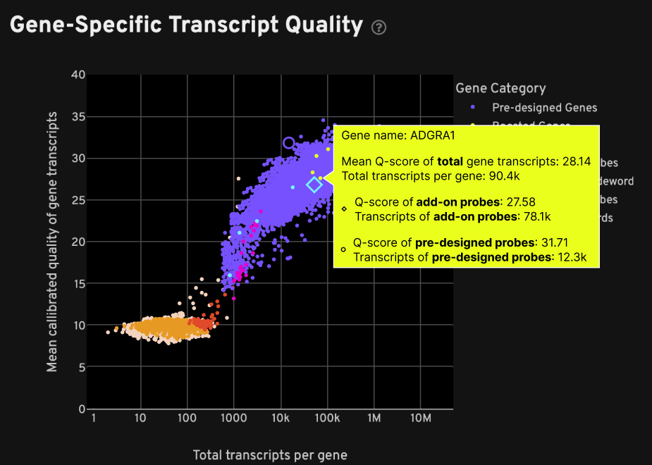
Both plots on the Decoding tab include a category called "Boosted Genes". In particular, the Gene-Specific Transcript Quality plot shows the breakdown of mean Q-Score and total transcript information, which help to assess added probe performance, when hovering over the boosted gene point on the plot. For the example below, the mean Q-Score and total transcripts metrics are shown per gene for:
- Total: the combined result from add-on + pre-designed probe sets
- Add-on probe sets: the added probe sets result alone (light blue diamond icon)
- Pre-designed probe sets: the original pre-designed probe sets result alone (purple circle icon)
In this example, gene boosting added 78.1k transcripts for this gene:

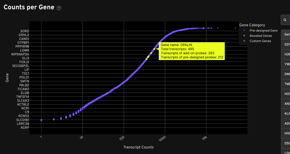
The Counts per Gene plot also indicates the number of transcripts from add-on probe sets and pre-designed probe sets. In this example, gene boosting added 283 transcripts for this gene:

The metrics in the Decoding tab Decoding Yield and Cell Segmentation tab Segmentation Metrics include separate metrics for pre-designed genes and custom genes. If boosted genes are present, transcripts from boosted genes are included in the pre-designed gene metrics. For example:
- The
median predesigned transcripts per cellmetric is calculated as the median number of high-quality (Q >= 20) transcripts per cell from pre-designed genes (10x-designed) and boosted genes (pre-designed genes for which extra probe sets were added). - The
median custom transcripts per cellmetric does not include counts from boosted genes.
To assess add-on probe performance further, use the codeword_category column (2nd to last column) in the transcripts.parquet file. You can examine information for transcripts (predesigned_gene) targeted by the pre-designed probes vs. transcripts (custom_gene) targeted by the added probes.
Add-on probe performance can be assessed with the plots and metrics described above in the analysis_summary.html and the transcripts.parquet file for XOA v3.2 outputs. For XOA v3.0 - 3.1 data, you can examine the transcripts.parquet file to distinguish the contributions from pre-designed vs. added probes.
import dask.dataframe as dd # Read in the parquet file, edit path to where parquet file saved df = dd.read_parquet('transcripts.parquet') # Print information about the data frame df.info() # Print first 5 rows of the dask data frame df.head() # Subset by the boosted gene, example is IL1B boosted_genes = df[df['feature_name'] == 'IL1B'] print(boosted_genes.compute()) # save the subset as a CSV boosted_genes.to_csv('subset_IL1B_transcript_info', index=False)
The subset CSV file looks something like this (scroll right to see the codeword_category distinction):
transcript_id,cell_id,overlaps_nucleus,feature_name,x_location,y_location,z_location,qv,fov_name,nucleus_distance,codeword_index,codeword_category,is_gene 281474976719863,fajfmnbb-1,0,IL1B,37.453125,64.5625,19.09375,40.0,Y12,3.046875,383,predesigned_gene,True 281474976719903,fbifjjcc-1,0,IL1B,64.46875,110.28125,15.3125,30.25,Y12,1.140625,383,predesigned_gene,True 281474976719934,fcknkoij-1,0,IL1B,83.65625,125.328125,15.4375,40.0,Y12,0.28125,383,predesigned_gene,True 281474976719949,fclbhomd-1,1,IL1B,92.5,122.328125,17.171875,40.0,Y12,0.0,383,predesigned_gene,True 281474976719954,fclbhomd-1,0,IL1B,93.328125,122.734375,18.46875,40.0,Y12,0.265625,383,predesigned_gene,True ... 281474976710687,fchcbdda-1,0,IL1B,7.078125,227.125,14.75,40.0,Y12,1.78125,416,custom_gene,True 281474976710696,faljlgoo-1,0,IL1B,10.140625,39.546875,15.0,40.0,Y12,1.421875,416,custom_gene,True 281474976710741,fahehfcf-1,0,IL1B,15.890625,53.890625,18.765625,40.0,Y12,1.703125,416,custom_gene,True 281474976710771,faflhkgm-1,0,IL1B,20.3125,23.359375,17.0,40.0,Y12,1.578125,416,custom_gene,True 281474976710773,UNASSIGNED,0,IL1B,18.171875,246.78125,18.03125,40.0,Y12,5.765625,416,custom_gene,True 281474976710783,fahklcna-1,0,IL1B,20.453125,102.78125,18.796875,40.0,Y12,3.453125,416,custom_gene,True ...