This guide outlines a fast and lightweight approach to optimize cellpose3 (preprint, github, documentation) parameters for its existing cyto3 model to segment large cells or cells that are unfamiliar to 10x segmentation models. This approach applies to a single fluorescence image where the stain clearly shows the boundaries of the cell type or structure of interest. It is meant to quickly rescue cells of interest and shows how to produce a numpy NPY file compatible with the import-segmentation pipeline of Xenium Ranger. The approach does not train a custom model, which became a feature in cellpose2, nor does it use the desktop GUI version of cellpose3.

The Xenium Multimodal Cell Segmentation (MCS) software algorithm efficiently defines cell boundaries based on stains of biological features and prior model training of cell features. The models, currently on v3, perform suboptimally (i) on large structures or cell types with a diameter larger than 100 µm (e.g. muscle, adipocytes, and signet ring cells) and (ii) on unusual cell types such as dorsal root ganglion where nuclei stain weakly. The MCS fluorescence stains distinctly define these cell boundaries.

• Xenium segmentation model training is continuous and Xenium Ranger will enable applying improvements to older data.
• For other approaches to rescuing Xenium transcripts outside of cells, see here.

Testing on adipocytes, skeletal muscle¹, dorsal root ganglion^1,2, and signet ring cells¹ shows the approach can quickly derive parameters that can rescue a fair proportion of these cell types. Rescued shapes include jagged muscle cross sections and medium-length muscle longitudinal sections. Long longitudinal muscle structures remain challenging. Manual annotation of such structures may be the fastest way forward for researchers with few samples. For many samples, consider custom model training.

Specifically, the guide illustrates by defining adipocytes from the Xenium Prime 5K human lymph node sample public data set (Figures 3–5). We use a small ground truth annotation GeoJSON and its small region of the image to test different image resolutions and cell diameters in cellpose3. The code filters the results from the parameters based on area overlap and number of polygons. The code applies selected parameters on the full image and saves a full-resolution scale result to numpy (NPY). The guide goes on to show how to compare the coverage of the cellpose3 mask to that of the Xenium cell mask, as well as estimate the fraction of transcripts the cellpose3 mask rescues using the Xenium transcripts.parquet result.

Figure 1: Cellpose3 mask results from various cell types for the small test regions and chosen parameterizations.

Figure 2: Cellpose3 mask results from various cell types. Left image is a binary representation of tissue stain with manually drawn ground truth polygons overlaid in red. Right image is the cellpose3 mask result. A. Adipocytes of lymph node tissue. B. Muscle tissue with both cross and longitudinal sections. C. Dorsal root ganglion (DRG). D. Signet ring cells (SRC). Some images were subset.

Table 1: Cellpose3 stain image, parameters, and metrics for various cell types.

Figure 3: Lymph node sample. The alpha-SMA/Vimentin interior protein stain is green across the images. It is faint in the composite image, and the single-channel image adjusts the channel intensity threshold to enhance the visibility of the signal. The XOA v3.0 and cellpose3 images show the cell boundaries in white outline from the Xenium Onboard Analysis pipeline and the Xenium Ranger import-segmentation run that uses the cellpose3 mask, respectively. The rightmost image shows ADIPOQ transcripts, a marker of adipocytes, in a scaled view in pink. Visualization performed in Xenium Explorer v3.1.1.

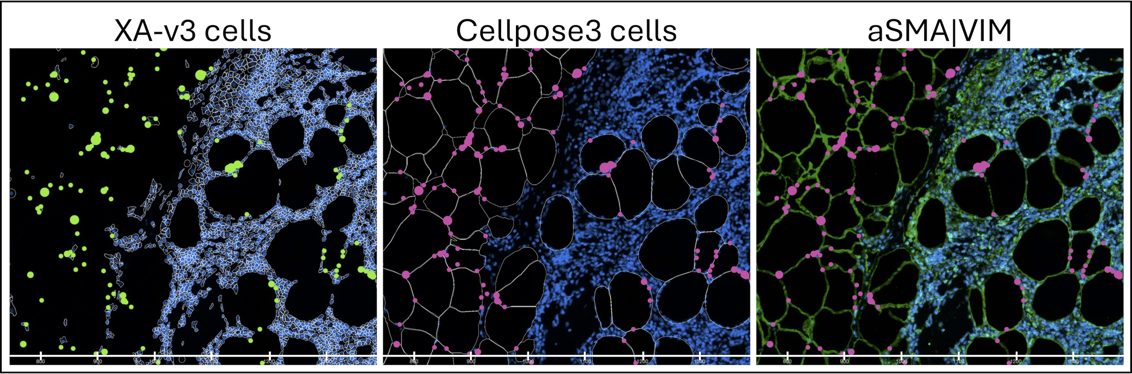
Figure 4: Lymph node sample zoomed view where x-axis markers denote a 100 µm span. DAPI is in blue across the images, and cell outlines are in white for the Xenium Onboard Analysis (XOA) v3.0 and cellpose3 images. The third image shows alpha-SMA|VIM staining in green. ADIPOQ transcript is in an aggregated scaled view and displays as green circles in XOA v3.0 and pink circles in the cellpose3 result. Visualization performed in Xenium Explorer v3.1.1.

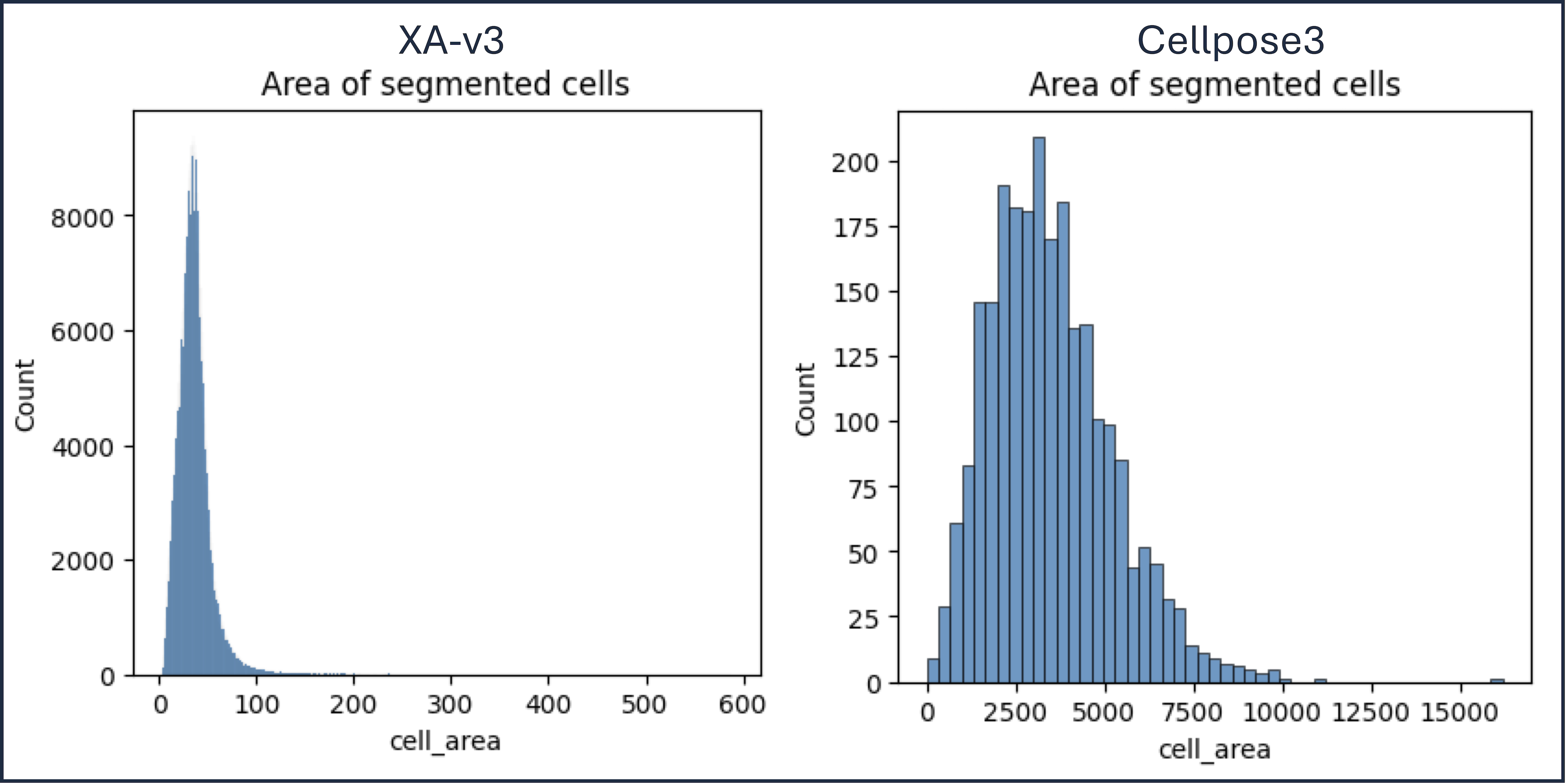
Figure 5: Lymph node sample. The area (µm²) of cellpose3 cells is much larger than XOA v3.0 cells. The result used a cellpose diameter of 75 µm, which for a circle gives an area of 4,418 µm².

1. Fluorescence image registered to Xenium data, e.g. MCS stain image.

   • The tutorial segments adipocytes for a public data set, the Xenium Prime 5K human lymph node sample, using the alphaSMA/Vimentin interior protein stain image corresponding to the morphology_focus/morphology_focus_0003.ome.tif layer. This stain highlights structural features and is currently unused by the Xenium Multimodal Cell Segmentation pipeline.
   • Note the adipocytes surrounding the main lymph node tissue present few transcripts. Transcript rescue by assignment to cell definitions can be one goal of custom segmentation. Another goal may be to analyze spatial features of the cells, e.g. size and distribution pattern.

2. QuPath and 10 minutes to manually annotate polygons for a small region of the image.

   • Load the full image into QuPath and annotate features of interest for a small region. Select a region that represents the variety of the target cell sizes if the features vary in size, and consider including undesirable features to exclude parameters that pick up on the unwanted features.
   • See this video tutorial on creating annotations in QuPath. Use the polygon tool to avoid creating multipolygons and other more complex annotations.
   • Save the annotations as a geojson (File > Export objects as GeoJSON > Export > All objects).
   • The discussion section of the article here shows a polygon annotation for a small region of the lymph node sample. Download the premade ground truth GeoJSON from here. Use the default annotation thickness.

3. An estimated range for cell or structure diameters in microns

4. (Optional) Xenium cells.zarr.zip and transcripts.parquet results for metrics calculations

5. (Optional) Linux system with Xenium Ranger installed. Guide illustrations use v3.0. To download Xenium Ranger and for system requirements, see here.

   • If you downloaded the preview lymph node data prior to November 14, 2024, please replace the output bundle's gene_panel.json with the file available on the data page before running import-segmentation.

6. Python3. This guide was tested using the following package versions (example installation with conda):

   Copy
   conda create -n cellpose-env cellpose==3.0.10 geopandas==1.0.1 numpy==1.26.4 pandas==2.2.2 scikit-image==0.24.0 scipy==1.14.0 shapely==2.0.5 tifffile==2024.7.24 zarr==2.18.2
   

1.1. Load packages and configure cellpose3.

Copy
import cellpose
import geopandas as gpd
import numpy as np
import pandas as pd
import scipy
import shapely
import skimage as ski
import tifffile
import zarr

from cellpose import core, utils, io, models, metrics, plot
from collections import Counter
from matplotlib import pyplot as plt
from shapely.geometry import Polygon
from tqdm import tqdm

# Allow cellpose to print stdout progress
io.logger_setup()

# Use cyto3 cellpose model
model = models.Cellpose(gpu=False, model_type='cyto3')

# Parameter to use single-image mode.
channels = np.array([[0,0]])

1.2. Define data locations and constants. Remember to edit the directory paths below to match the input file location on your computer.

Copy
# Input directory - ddir specifies the top data directory, fasmavim specifies the alphaSMA/Vimentin morphology image file, a1url specifies the lymph node directory path. Example paths shown below.
ddir = '/Users/soo.lee/Documents/data/'
fasmavim = 'morphology_focus/morphology_focus_0003.ome.tif'
a1url = f'{ddir}public-hu-lymph-node-5k/Xenium_Prime_Human_Lymph_Node_Reactive_FFPE_outs/{fasmavim}'
# Output directory
odir = f'{ddir}cellpose/'
gjurl = f'{odir}a.geojson'

# Levels: pixelsize in µm https://kb.10xgenomics.com/hc/en-us/articles/11636252598925
scalefactors = {
    0: 0.2125,
    1: 0.4250,
    2: 0.85,
    3: 1.7,
    4: 3.4,
    5: 6.8,
    6: 13.6,
    7: 27.2,
}

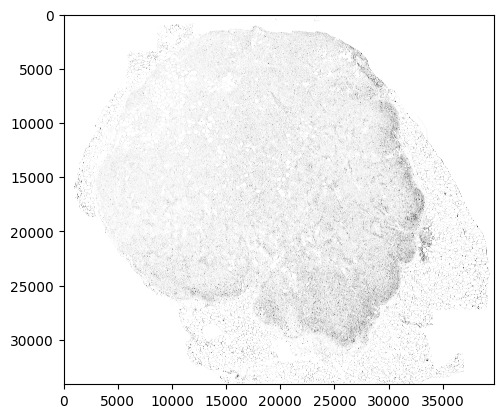
1.3. Load stain image and plot.

Copy
level = 0
pixelsize = scalefactors[level]
a = tifffile.imread(a1url, is_ome=False, level=level)
plt.imshow(a, cmap='binary')
plt.axis('scaled')
plt.show()

1.4. Load ground truth geojson and plot.

Copy
# Two ways to load: as pandas DataFrame or as GeoDataFrame. Run both to follow this guide.
gdf = pd.read_json(gjurl)
gj = gpd.read_file(gjurl)
gj.plot(facecolor='none', edgecolor='red', aspect=1)
plt.show()

How many polygons are in the ground truth mask? There are 57.

Copy
numtruthmasks = len(gdf)
numtruthmasks

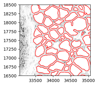
1.5. Plot the polygons over the stain image.

Copy
fig,ax = plt.subplots()
plt.imshow(a, cmap='binary')
gj.plot(ax=ax, facecolor='none', edgecolor='red', aspect=1)
plt.show()

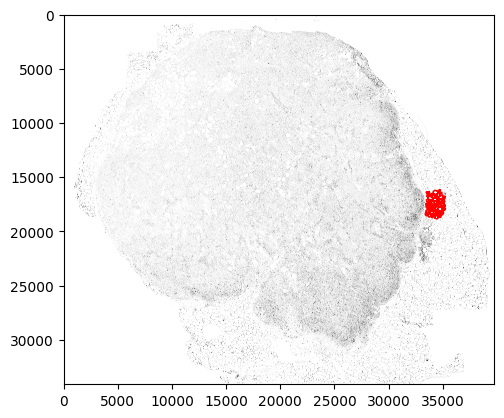
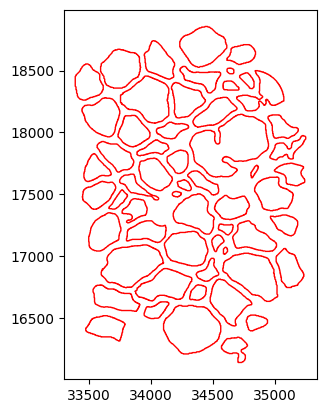
1.6. Define coordinates of the small region and plot to confirm.

Copy
ystart = 16500
yend = 18500
xstart = 33050
xend = 35050

plt.rcParams["figure.figsize"] = (3,3)
fig,ax = plt.subplots()
plt.imshow(a, cmap='binary')
gj.plot(ax=ax, facecolor='none', edgecolor='red', aspect=1)
plt.axis('scaled')
plt.ylim(ystart,yend)
plt.xlim(xstart,xend)
plt.show()

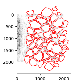
2.1. Subset the small test region and shift coordinates. Reuse code in [1.6] to plot to confirm.

Copy
subset = a[ystart:yend, xstart:xend]

# Wrangle GeoDataFrame
sgeoms = []
for i,row in gj.iterrows():
    sgeoms.append(shapely.affinity.translate(row['geometry'], xoff=-xstart, yoff=-ystart))
gj['geometry'] = sgeoms

# Wrangle DataFrame
sgeoms2 = []
for i,row in gdf.iterrows():
    pcoors = row.features['geometry']['coordinates'][0]
    v = np.array([xstart, ystart])
    result = [pcoors - v[:]]
    item = {'geometry': {'coordinates': result}}
    sgeoms2.append(item)
gdf['sgeoms'] = sgeoms2

2.2. Create a mask of the polygons.

Copy
mm = np.zeros(subset.shape)
for i,row in gdf.iterrows():
    p = np.array(row['sgeoms']['geometry']['coordinates']).squeeze()
    r,c = ski.draw.polygon(p[:,1],p[:,0], subset.shape)
    mm[r,c] = 1

2.3. Define downsample levels and diameters in microns to test.

Copy
factors = [0,1,2,3]
diameters = [50, 75, 100] #µm

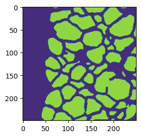
2.4. Create downsampled versions of the mask and stain image.

Copy
dmasks = {}
for factor in factors:
    dm = scipy.ndimage.zoom(mm, pixelsize/scalefactors[factor])
    dmasks[factor] = dm

# Plot the last downsampled mask
plt.imshow(dm)

Print the image factors and shape:

Copy
images = {}
for factor in factors:
    img = scipy.ndimage.zoom(subset, pixelsize/scalefactors[factor])
    images[factor] = img
    print(factor, img.shape)

# The output should look like this:
#0 (2000, 2000)
#1 (1000, 1000)
#2 (500, 500)
#3 (250, 250)

3.1. Run cellpose3 on the combinations of downsampled image and diameter length. Four resolutions and three diameters gives twelve combinations.

Copy
results = {}
for diameter in diameters:
    results[diameter] = {}

    for factor,img in images.items():
        # Rescale micron diameter to match image pixels
        diam = round(diameter/(scalefactors[factor]), 0)
        print(factor, diameter, diam)

        # Run cellpose3
        masks,flows,styles,diams = model.eval(img, diameter=diam, channels=channels)
        results[diameter][factor] = [masks,flows,styles,diams]

# The output should look like this:
#0 50 235.0
#2024-10-24 14:57:48,367 [INFO] channels set to [[0 0]]
#2024-10-24 14:57:48,370 [INFO] ~~~ FINDING MASKS ~~~
#2024-10-24 14:59:43,773 [INFO] >>>> TOTAL TIME 115.41 sec
#1 50 118.0
#2024-10-24 17:29:39,660 [INFO] channels set to [[0 0]]
#2024-10-24 17:29:39,661 [INFO] ~~~ FINDING MASKS ~~~
#2024-10-24 17:29:51,416 [INFO] >>>> TOTAL TIME 11.76 sec
#…
#3 100 59.0
#2024-10-24 15:06:20,259 [INFO] channels set to [[0 0]]
#2024-10-24 15:06:20,259 [INFO] ~~~ FINDING MASKS ~~~
#2024-10-24 15:06:20,641 [INFO] >>>> TOTAL TIME 0.38 sec

The full-resolution image takes roughly 10x more time to run than the next resolution image. Even if it produces the best segmentation results, this should count against choosing it over the reduced run times of lower resolution images.

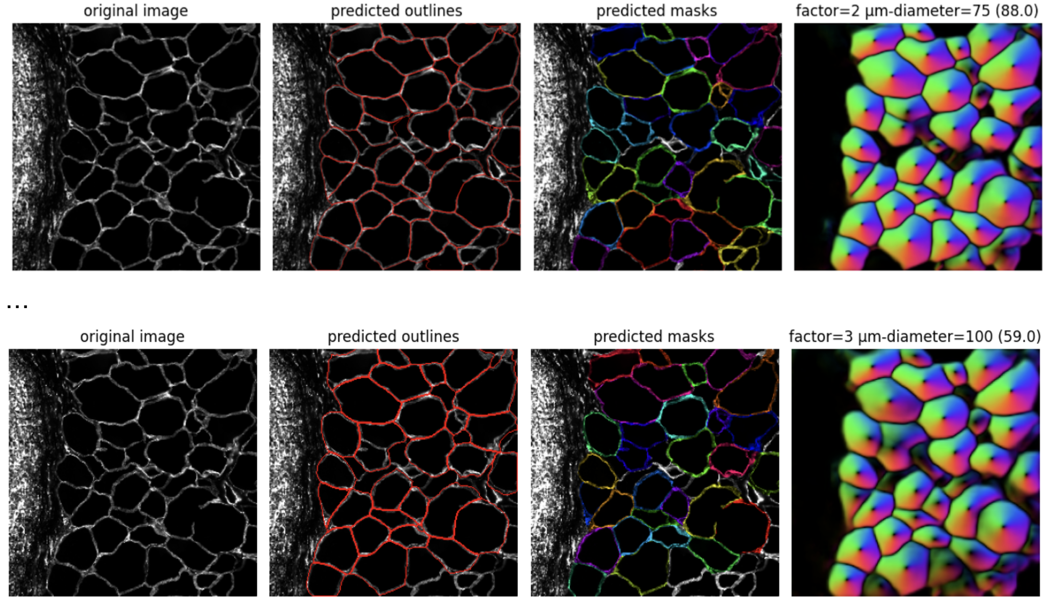
3.2. Visualize results using cellpose3 plotting function plot.show_segmentation. Each row represents one condition.

Copy
for diameter,result in results.items():
    for factor,r in result.items():
        masks,flows,styles,diams = r
        fig = plt.figure(figsize=(12,5))
        plot.show_segmentation(fig, images[factor], masks, flows[0], channels=channels[0])
        plt.tight_layout()
        plt.title(f'factor={factor} µm-diameter={diameter} ({diams})')
        plt.show()

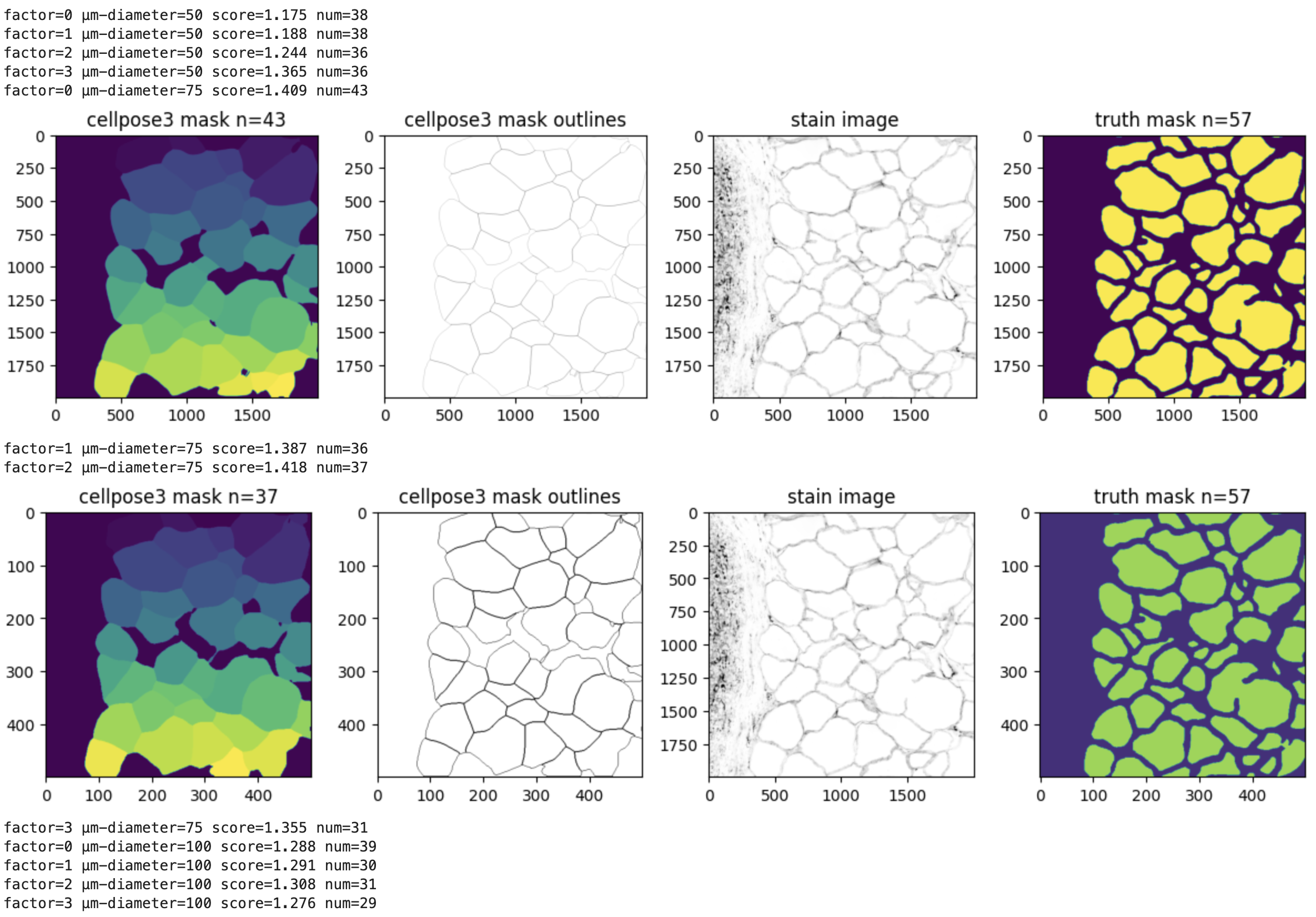
3.3. Calculate the fraction overlap and compare the number of polygons against the ground truth mask.

Copy
for diameter,result in results.items():
    for factor,r in result.items():
        masks,flows,styles,diams = r
        truthmask = dmasks[factor]
        intersection_mask = np.logical_and(masks, truthmask)

        # Fraction overlap
        score = round(np.sum(intersection_mask)/np.sum(truthmask),3)
        # Number of polygons
        nummasks = len(Counter(masks.flatten())) - 1
        print(f'factor={factor} µm-diameter={diameter} score={score} num={nummasks}')

        # Configure cutoffs and plot those passing muster
        if ((score < 1.6) and (score > 1.4) and
            (nummasks <=numtruthmasks*1) and (nummasks >=numtruthmasks/1.6)):
            fig, axs = plt.subplots(1, 4, figsize=(12, 3))
            axs[0].imshow(masks)
            axs[0].set_title(f'cellpose3 mask n={nummasks}')
            axs[1].imshow(utils.masks_to_outlines(masks), cmap='binary')
            axs[1].set_title('cellpose3 mask outlines')
            axs[2].imshow(subset, cmap='binary')
            axs[2].set_title('stain image')
            axs[3].imshow(truthmask)
            axs[3].set_title(f'truth mask n={numtruthmasks}')
            plt.tight_layout()
            plt.show()

4.1. Define parameters for full image run. These are the parameters from cellpose3 mask n=37.

Copy
factor = 2
diameter = 75

4.2. Run cellpose3 with chosen parameters on the full image.

Copy
img = scipy.ndimage.zoom(a, pixelsize/scalefactors[factor])
diam = round(diameter/(scalefactors[factor]), 0)
masks2,flows2,styles2,diams2 = model.eval(img, diameter=diam, channels=channels)

# The output should look like this
#2024-10-24 19:44:17,530 [INFO] channels set to [[0 0]]
#2024-10-24 19:44:17,530 [INFO] ~~~ FINDING MASKS ~~~
#2024-10-24 19:48:36,310 [INFO] >>>> TOTAL TIME 258.78 sec

That was not long at all. Check the number of polygons. There are 2,436 polygons.

Copy
numcells = len(set(masks2.flatten())) - 1
numcells

Visualize the results using cellpose3 plotting function plot.show_segmentation. This can take some time to render, so consider skipping in favor of the larger plot in the next step.

Copy
fig = plt.figure(figsize=(12,5))
plot.show_segmentation(fig, img, masks2, flows2[0], channels=channels[0])
plt.tight_layout()
plt.show()

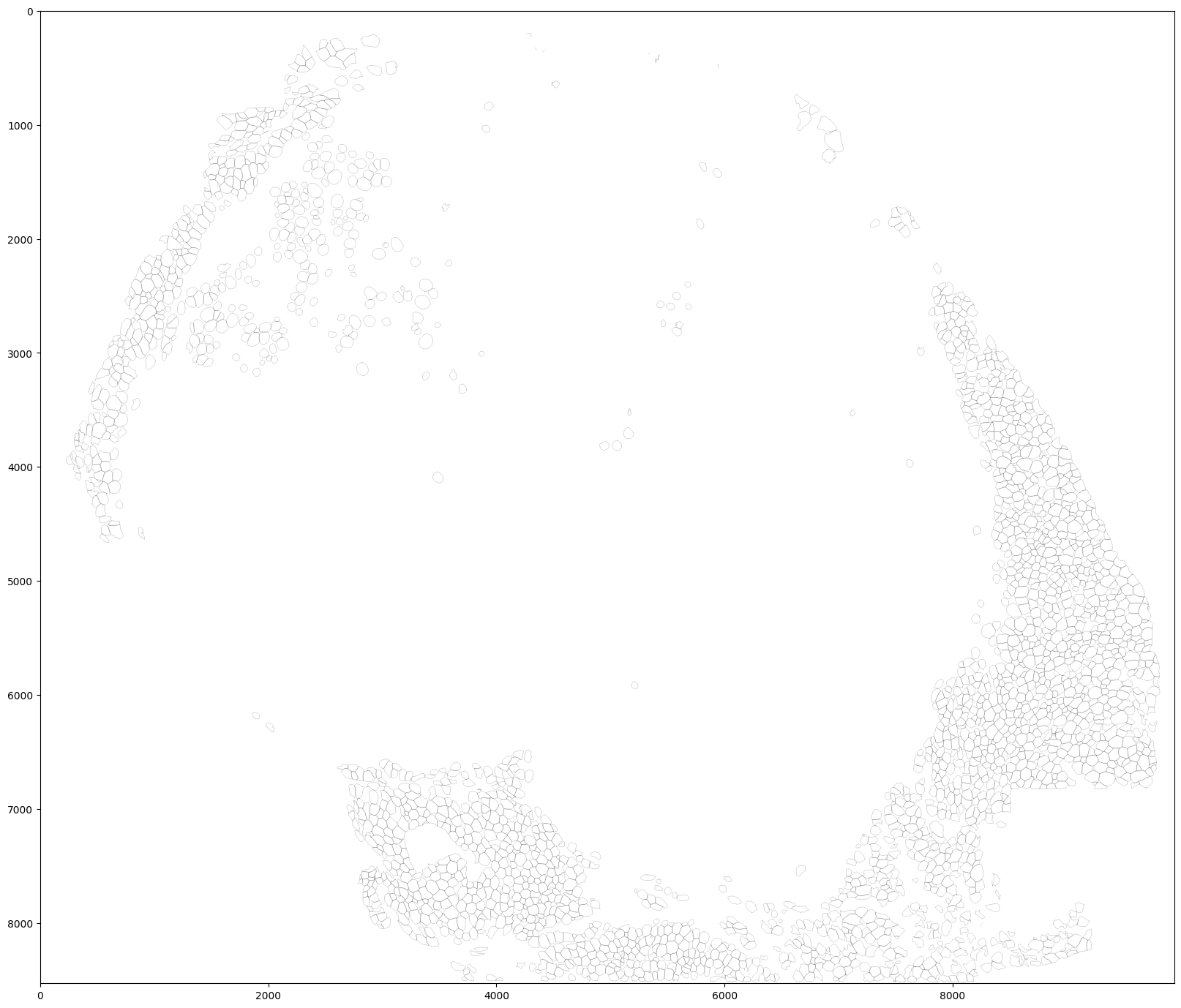
Visualize the mask outlines.

Copy
plt.rcParams["figure.figsize"] = (20,20)
plt.imshow(utils.masks_to_outlines(masks2), cmap='binary')

5.1. Scale the mask to the highest resolution image scale.

Copy
resampled_mask = ski.transform.resize(masks2, a.shape, order=0, preserve_range=True, anti_aliasing=False)
resampled_mask.shape
#Output: (34119, 39776)

5.2. Save to numpy NPY format file for use with Xenium Ranger. This produces a 2.71GB file.

Copy
np.save(f'{odir}a.npy', resampled_mask, allow_pickle=True)

5.3. (Optional) Run with the Xenium Ranger v3.0 and later import-segmentation pipeline on a Linux system. Remember to edit the directory paths below to match the input file locations on your computer.

Copy
xeniumranger import-segmentation \
             --id xr30is-a-npy \
             --xenium-bundle /Xenium_Prime_Human_Lymph_Node_Reactive_FFPE_outs/ \
             --cells a.npy \
             --localcores 32 \
             --localmem 128

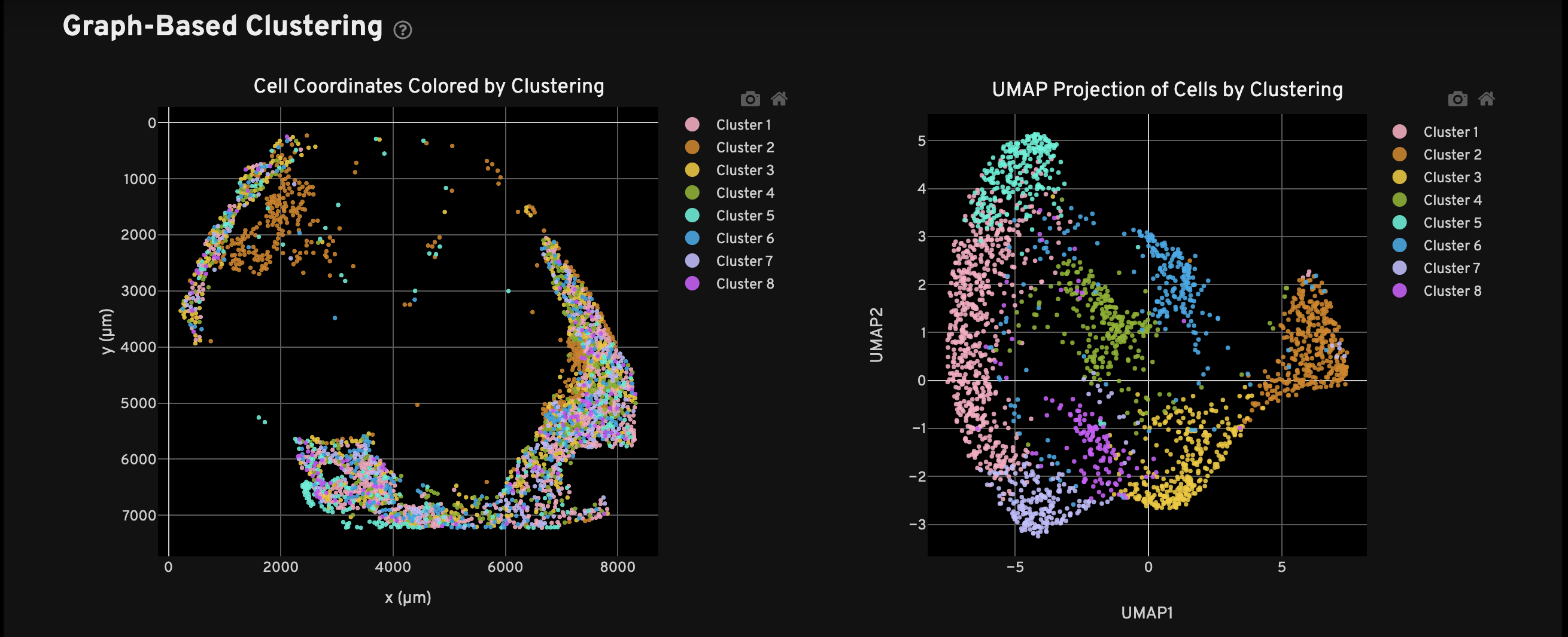
The run assigns 1.0% of transcripts (~2M) to 2,436 cells that add 33% more tissue coverage. Graph-based clustering produces eight clusters with differentially expressed genes known to be expressed in adipocytes including ADIPOQ, AQP7, CIDEC, LEP, and PLIN4.

Quantify the impact of the cellpose3 rescue using the cellpose3 mask and existing Xenium results, specifically the transcripts and the Xenium cell masks.

6.1. Load transcripts and cell mask. Remember to edit the directory paths below to match the input file location on your computer.

Copy
#Input directory
lymphurl = f'{ddir}public-hu-lymph-node-5k/Xenium_Prime_Human_Lymph_Node_Reactive_FFPE_outs/'
turl = f'{lymphurl}transcripts.parquet'
murl = f'{lymphurl}cells.zarr.zip'

# Load the transcripts into pandas DataFrame. This takes a while.
t = pd.read_parquet(turl)
ttotal = len(t)
print(ttotal)
#Output: 232650139

# Load the XOA cell mask. mask_index=0 is nuclei and mask_index=1 is cells.
z = zarr.open(murl, mode="r")
cmask = z['masks']['1'][:]
cmask.shape
#Output: (34119, 39776)

6.2. The transcript ZYX coordinates are in µm units. Add pixel coordinates.

Copy
f = scalefactors[0]
t['x'] = round(t['x_location']/f, 0)
t['y'] = round(t['y_location']/f, 0)

6.3. Subsample to 1% of the transcripts for faster estimations and count the fraction of transcripts not captured by Xenium cells. The subsampled table gives 0.054 fraction of cells unassigned to a cell.

Copy
tsub = t.sample(frac=0.01).copy(deep=True)
print(len(tsub))
#Output: 2326501

# Fraction transcripts not captured by cells
len(tsub[tsub['cell_id'] == 'UNASSIGNED'])/len(tsub)
#Output: 0.054067030274218664

6.4. Tally transcripts in and out of the Xenium cell mask.

Copy
results = []
for i,row in tqdm(tsub.iterrows()):
    x = int(row['x'])
    y = int(row['y'])
    results.append(cmask[y,x] > 0)

#Output: 2326501it [00:42, 54470.81it/s]

Confirm the fraction not in the mask is the same as the fraction UNASSIGNED. We see a similar 0.054 fraction of transcripts not in cells.

Copy
r = dict(Counter(results))
r[False]/len(tsub)
#Output: 0.054025336761084564

6.5. Tally transcripts in and out of the cellpose3 mask.

Copy
results2 = []
for i,row in tqdm(tsub.iterrows()):
    x = int(row['x'])
    y = int(row['y'])
    results2.append(resampled_mask[y,x] > 0)

#Output: 2326501it [00:42, 55188.62it/s]

We expect the fraction transcripts not in the cellpose3 mask to be large and indeed it is 0.99.

Copy
r2 = dict(Counter(results2))
r2[False]/len(tsub)
#Output: 0.9903326927433085

The number of transcripts in the cellpose3 mask is ~2.2M, which is not insignificant.

Copy
round(ttotal*r2[True]/len(tsub), 0)
#Output: 2249100.0

6.7. Add both results to the subsampled dataframe.

Copy
tsub['results'] = results
tsub['results2'] = results2

The fraction of transcripts captured by both approaches (Xenium and cellpose3) is 0.0071.

Copy
len(tsub[(tsub['results'] == True) & (tsub['results2'] == True)])/len(tsub)
#Output: 0.00706726539124634

The estimated number of previously unassigned transcripts cellpose3 now assigns to cells is 604,900.

Copy
round(ttotal*len(tsub[(tsub['results'] == False) & (tsub['results2'] == True)])/len(tsub), 0)
#Output: 604900.0

These metrics paint a partial picture of improvements. Visual inspection shows the better quality of the cellpose3 segmentation, where adipocytes are fully defined and not fragmented.

6.8. Compare Xenium versus cellpose3 generated cell masks.

Copy
# Mask overlap mask
intersection = np.logical_and(resampled_mask, cmask)

# Merge of masks
union = np.logical_or(resampled_mask, cmask)

Fraction area overlap between the two pipeline runs is 0.01.

Copy
overlap = np.sum(intersection)/np.sum(union)
overlap
#Output: 0.010981660049060987

How much new area does the cellpose3 mask add?

Copy
xoaarea = np.count_nonzero(cmask)
cellposearea = np.count_nonzero(resampled_mask)
print(xoaarea, cellposearea)
#Output: 561000645 186800400

print(round((cellposearea-cellposearea\*overlap)/(xoaarea), 4))
#Output: 0.3293

The cellpose3 segmentation adds 33% more cell area coverage to the XOA results.

1. Muscle, dorsal root ganglion, and signet ring cell sample images graciously provided by researchers. Muscle data provided by service provider BIA Separations CRO, Labena d.o.o.
2. Dorsal root ganglion project was supported by the Single Cell Genomics Core at Baylor College of Medicine with funding from the CPRIT RP200504 and the NIH S10OD032189.

Code developed by Soo Hee Lee based upon data generated by the NIH Human BioMolecular Atlas Program (HuBMAP). The Human Body at Cellular Resolution: the NIH Human BioMolecular Atlas Program (doi:10.1038/s41586-019-1629-x).