Note: 10x Genomics does not provide support for community-developed tools and makes no guarantees regarding their function or performance. Please contact tool developers with any questions. If you have feedback about Analysis Guides, please email analysis-guides@10xgenomics.com.
As discussed in the Integrating Single Cell and Visium Spatial Gene Expression data Analysis Guide, several software tools have been developed for cell type deconvolution analysis of spatial transcriptomic datasets using single cell reference data. In a recent software benchmarking study, Li et al. (2022) showed that the R package spacexr (Cable et al. 2022) performed well across a variety of public and simulated datasets.
The purpose of this guide is to demonstrate how to use spacexr to integrate 10x Genomics single cell (Chromium) and spatial (Visium) gene expression data starting from Cell Ranger and Space Ranger software outputs.
Prerequisites:
- Linux system to run Space Ranger and Cell Ranger
- Space Ranger (tested on v1.3, v2.0)
- Cell Ranger (tested on v7.0)
- R (v4.0.3+)
For this example, we create the cell type reference from a Chromium 3' Single Cell Gene Expression mouse brain nuclei dataset to deconvolve cell types per spot in a Visium for FFPE mouse brain spatial dataset. To follow along, either A) download the input FASTQ files or B) download Space Ranger and Cell Ranger outputs from the 10x Genomics public datasets page. Run the following code in a Linux environment.
Create the working directory:
mkdir adult_mouse_brain_FFPE
mkdir adult_mouse_brain_SC
A) Download input FASTQ files
Download the mouse reference and FASTQ files for Visium and Chromium data into this directory:
- The 10x mouse reference genome is available on Cell Ranger or Space Ranger download pages.
# Download reference
curl -O https://cf.10xgenomics.com/supp/spatial-exp/refdata-gex-mm10-2020-A.tar.gz
# Untar the reference
tar -xf refdata-gex-mm10-2020-A.tar.gz
# Change directory to adult_mouse_brain_FFPE
cd adult_mouse_brain_FFPE
# Download visium inputs
curl -O https://cf.10xgenomics.com/samples/spatial-exp/1.3.0/Visium_FFPE_Mouse_Brain/Visium_FFPE_Mouse_Brain_fastqs.tar
curl -O https://cf.10xgenomics.com/samples/spatial-exp/1.3.0/Visium_FFPE_Mouse_Brain/Visium_FFPE_Mouse_Brain_image.jpg
curl -O https://cf.10xgenomics.com/samples/spatial-exp/1.3.0/Visium_FFPE_Mouse_Brain/Visium_FFPE_Mouse_Brain_probe_set.csv
# Untar the FASTQs
tar -xf Visium_FFPE_Mouse_Brain_fastqs.tar
# Change directory from adult_mouse_brain_FFPE to adult_mouse_brain_SC
cd ../adult_mouse_brain_SC
# Download FASTQs
curl -O https://cf.10xgenomics.com/samples/cell-exp/7.0.0/5k_mouse_brain_CNIK_3pv3/5k_mouse_brain_CNIK_3pv3_fastqs.tar
# Untar the FASTQs
tar -xf 5k_mouse_brain_CNIK_3pv3_fastqs.tar
The input working directory should look like:
├── adult_mouse_brain_FFPE
│ ├── Visium_FFPE_Mouse_Brain_fastqs
│ ├── Visium_FFPE_Mouse_Brain_image.jpg
│ └── Visium_FFPE_Mouse_Brain_probe_set.csv
├── adult_mouse_brain_SC
│ └── 5k_mouse_brain_CNIK_3pv3_fastqs
└── refdata-gex-mm10-2020-A
B) Download outputs from public datasets page
Alternatively, you can download the Visium and Chromium outputs from the 10x Genomics public datasets page. After downloading the files below, skip to step 5.
- For the Visium dataset (analyzed with Space Ranger v1.3):
# Change directory to adult_mouse_brain_FFPE
cd adult_mouse_brain_FFPE
# Download these files
curl -O https://cf.10xgenomics.com/samples/spatial-exp/1.3.0/Visium_FFPE_Mouse_Brain/Visium_FFPE_Mouse_Brain_filtered_feature_bc_matrix.h5
curl -O https://cf.10xgenomics.com/samples/spatial-exp/1.3.0/Visium_FFPE_Mouse_Brain/Visium_FFPE_Mouse_Brain_spatial.tar.gz
# Untar the spatial.tar.gz file, there should be a spatial/ directory that contains the tissue_positions_list.csv file
tar -xf Visium_FFPE_Mouse_Brain_spatial.tar.gz
# Rename the feature-barcode matrix file so it is recognized by the spacexr data input function
mv Visium_FFPE_Mouse_Brain_filtered_feature_bc_matrix.h5 filtered_feature_bc_matrix.h5
- For the Chromium dataset (analyzed with Cell Ranger v7.0):
# Change directory from adult_mouse_brain_FFPE to adult_mouse_brain_SC
cd ../adult_mouse_brain_SC
# Download this file
curl -O https://cf.10xgenomics.com/samples/cell-exp/7.0.0/5k_mouse_brain_CNIK_3pv3/5k_mouse_brain_CNIK_3pv3_filtered_feature_bc_matrix.h5
The input working directory should look like:
├── adult_mouse_brain_FFPE
│ ├── filtered_feature_bc_matrix.h5 #this is the renamed visium feature-barcode matrix file
│ └── spatial
│ ├── aligned_fiducials.jpg
│ ├── detected_tissue_image.jpg
│ ├── scalefactors_json.json
│ ├── tissue_hires_image.png
│ ├── tissue_lowres_image.png
│ └── tissue_positions_list.csv #this is the v1.3 coordinates file, note it is called tissue_positions.csv in v2.0
└── adult_mouse_brain_SC
└── 5k_mouse_brain_CNIK_3pv3_filtered_feature_bc_matrix.h5 #this is the SC feature-barcode matrix file
Run Cell Ranger in a Linux environment (computing options here). Warning: By default, Cell Ranger will use all of the cores available on your system to execute pipeline stages. See cellranger count documentation for additional options.
If you downloaded the FASTQ files, set up and run the Cell Ranger command below (be sure to edit /path/to/):
cellranger count --id=5k_adult_mouse_brain_SC_RUN1 \
--transcriptome=/path/to/refdata-gex-mm10-2020-A \
--fastqs=/path/to/adult_mouse_brain_SC/5k_mouse_brain_CNIK_3pv3_fastqs
Run Space Ranger in a Linux environment (computing options here). Warning: By default, Space Ranger will use all of the cores available on your system to execute pipeline stages. See spaceranger count documentation for additional options.
If you downloaded the FASTQ files, set up and run the Space Ranger command below (be sure to edit /path/to/):
spaceranger count --id=Visium_FFPE_Mouse_Brain_RUN1 \
--transcriptome=/path/to/refdata-gex-mm10-2020-A \
--probe-set=/path/to/adult_mouse_brain_FFPE/Visium_FFPE_Mouse_Brain_probe_set.csv \
--fastqs=/path/to/adult_mouse_brain_FFPE/Visium_FFPE_Mouse_Brain_fastqs \
--image=/path/to/adult_mouse_brain_FFPE/Visium_FFPE_Mouse_Brain_image.jpg \
--slide=V11J26-127 \
--area=B1
The rest of this guide will be done in R. If you are running the R analysis on a different system (e.g., local computer) than the one used to generate Cell Ranger and Space Ranger outputs (e.g., cluster), you'll need to download, at minimum, the following files:
├── adult_mouse_brain_FFPE
│ ├── filtered_feature_bc_matrix.h5 #the visium feature-barcode matrix file
│ └── spatial
│ └── tissue_positions.csv #for SRv2.0, or tissue_positions_list.csv for SRv1.3
└── adult_mouse_brain_SC
└── filtered_feature_bc_matrix.h5 #the chromium feature-barcode matrix file
Note that Space Ranger v1.3 tissue_positions_list.csv is the same as Space Ranger v2.0 tissue_positions.csv, the latter has column headers but the values are the same.
In R, install and load the following R packages:
# Install R packages (only need to do this once, or if you need to update packages)
install.packages("devtools")
devtools::install_github("dmcable/spacexr", build_vignettes = FALSE)
install.packages("Seurat")
install.packages("ggplot2")
# Load libraries
library(spacexr)
library(Seurat)
library(ggplot2) #for saving result plots
For the next steps, you'll need to know the path to the Cell Ranger and Space Ranger output files. The example code has placeholders /path/to/ that must be replaced to run; they have been written assuming the file structure shown in Step 2.
Spacexr requires two of the Space Ranger output files and the data structure/file names must look like this to use the read.VisiumSpatialRNA() function:
...
├── filtered_feature_bc_matrix.h5
└── spatial
└── tissue_positions.csv #for SRv2.0, or tissue_positions_list.csv for SRv1.3
The filtered_feature_bc_matrix.h5 file provides the gene-barcode count matrix information and the tissue_positions.csv provides the x-y coordinates for the spots on the tissue.
Optional: To match the orientation of the tissue on the slide with spacexr result plots, we will flip and mirror the coordinates:
# Read in the tissue_positions_list.csv file (path dependent on data download method from step 2)
vis_coords <- read.csv('/path/to/adult_mouse_brain_FFPE/Visium_FFPE_Mouse_Brain_RUN1/outs/spatial/tissue_positions.csv',
header=TRUE)
# Or if you downloaded the outputs from the 10x Genomics public datasets page:
#vis_coords <- read.csv('/path/to/adult_mouse_brain_FFPE/spatial/tissue_positions_list.csv',
# header=FALSE)
head(vis_coords)
# Col 3 is the x coord
# Col 4 is the y coord
The Space Ranger v2.0 tissue_positions.csv looks like this:
barcode in_tissue array_row array_col pxl_row_in_fullres pxl_col_in_fullres
1 ACGCCTGACACGCGCT-1 0 0 0 5247 21461
2 TACCGATCCAACACTT-1 0 1 1 5392 21208
3 ATTAAAGCGGACGAGC-1 0 0 2 5537 21461
4 GATAAGGGACGATTAG-1 0 1 3 5682 21208
5 GTGCAAATCACCAATA-1 0 0 4 5828 21460
6 TGTTGGCTGGCGGAAG-1 0 1 5 5972 21208
# Multiply x and y coordinates by -1 to flip/mirror
vis_coords[,3] <- vis_coords[,3]*-1
vis_coords[,4] <- vis_coords[,4]*-1
head(vis_coords)
The x-y coordinates are now flipped:
barcode in_tissue array_row array_col pxl_row_in_fullres pxl_col_in_fullres
1 ACGCCTGACACGCGCT-1 0 0 0 5247 21461
2 TACCGATCCAACACTT-1 0 -1 -1 5392 21208
3 ATTAAAGCGGACGAGC-1 0 0 -2 5537 21461
4 GATAAGGGACGATTAG-1 0 -1 -3 5682 21208
5 GTGCAAATCACCAATA-1 0 0 -4 5828 21460
6 TGTTGGCTGGCGGAAG-1 0 -1 -5 5972 21208
# Resave file.
# Note that due to the file name requirement, we will write over the original file with this new one
write.table(vis_coords, '/path/to/adult_mouse_brain_FFPE/Visium_FFPE_Mouse_Brain_RUN1/outs/spatial/tissue_positions.csv', quote=FALSE, row.names=FALSE, sep=',')
# Or if you downloaded the outputs from the 10x Genomics public datasets page:
#write.table(vis_coords[-1,], './adult_mouse_brain_FFPE/spatial/tissue_positions_list.csv',
# quote=FALSE, row.names=FALSE, col.names=FALSE, sep=',')
Now, we will use the read.VisiumSpatialRNA() function to read in the Visium data.
# Load Visium data directly from Space Ranger output directory
VisiumData<-read.VisiumSpatialRNA("/path/to/adult_mouse_brain_FFPE/Visium_FFPE_Mouse_Brain_RUN1/outs")
# Or if you downloaded the outputs from the 10x Genomics public datasets page:
#VisiumData<-read.VisiumSpatialRNA("/path/to/adult_mouse_brain_FFPE/")
The output message contains this warning; it is okay to continue.
Warning message:
In SpatialRNA(coords[, c("x", "y")], counts) :
SpatialRNA: some barcodes in nUMI, coords, or counts were not mutually shared. Such barcodes were removed.
# Create a list of barcodes from the column names of the count matrix
barcodes <- colnames(VisiumData@counts)
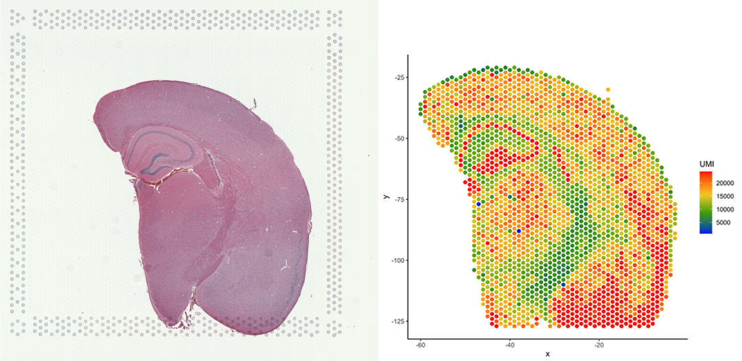
# Plot number of UMIs per barcode (spot)
plot_puck_continuous(puck=VisiumData, barcodes=barcodes, plot_val=VisiumData@nUMI,
size=1, ylimit=c(0,round(quantile(VisiumData@nUMI,0.9))),
title='plot of nUMI')
Note that this image now resembles the tissue on the slide (web summary slide image).

Spacexr requires the filtered_feature_bc_matrix.h5 output from Cell Ranger, as well as an annotation file with cell types for each barcode.
We are using Seurat to format the feature-barcode matrix information into a single count matrix for spacexr.
# Load single cell data from Cell Ranger output directory
Counts<-Read10X_h5("/path/to/adult_mouse_brain_SC/5k_adult_mouse_brain_SC_RUN1/outs/filtered_feature_bc_matrix.h5")
# Or if you downloaded the outputs from the 10x Genomics public datasets page:
#Counts<-Read10X_h5("/path/to/adult_mouse_brain_SC/5k_mouse_brain_CNIK_3pv3_filtered_feature_bc_matrix.h5")
# Create new Seurat Object from the count input
count_SeuratObject<-CreateSeuratObject(Counts)
# Create a count matrix object and take a look at the matrix
sc_counts <- count_SeuratObject@assays$RNA@counts
sc_counts[1:5,1:5]
5 x 5 sparse Matrix of class "dgCMatrix"
AAACCCAAGGCATCAG-1 AAACCCAAGGTTCACT-1 AAACCCACAAAGGCTG-1 AAACCCACAATGACCT-1 AAACCCACACGAGGAT-1
Xkr4 3 3 9 12 19
Gm1992 . . 1 . .
Gm19938 . . 3 1 .
Gm37381 . . . . .
Rp1 . . . . .
The cell type file can be generated manually with Loupe Browser using marker genes to assign barcodes to cell types or with reference databases.
In this guide, we will use the Azimuth app for reference-based single-cell analysis (Hao et al. 2021) to generate cell type annotations. To annotate the single cell mouse brain dataset, we will use the "Mouse - Motor Cortex" app (Yao et al. 2021; annotation details here). Note that there may be limitations to using a motor cortex cell type annotation reference for a whole brain sample and spot deconvolution results will be influenced by the reference used.
-
Go to the "Mouse - Motor Cortex" reference app.
-
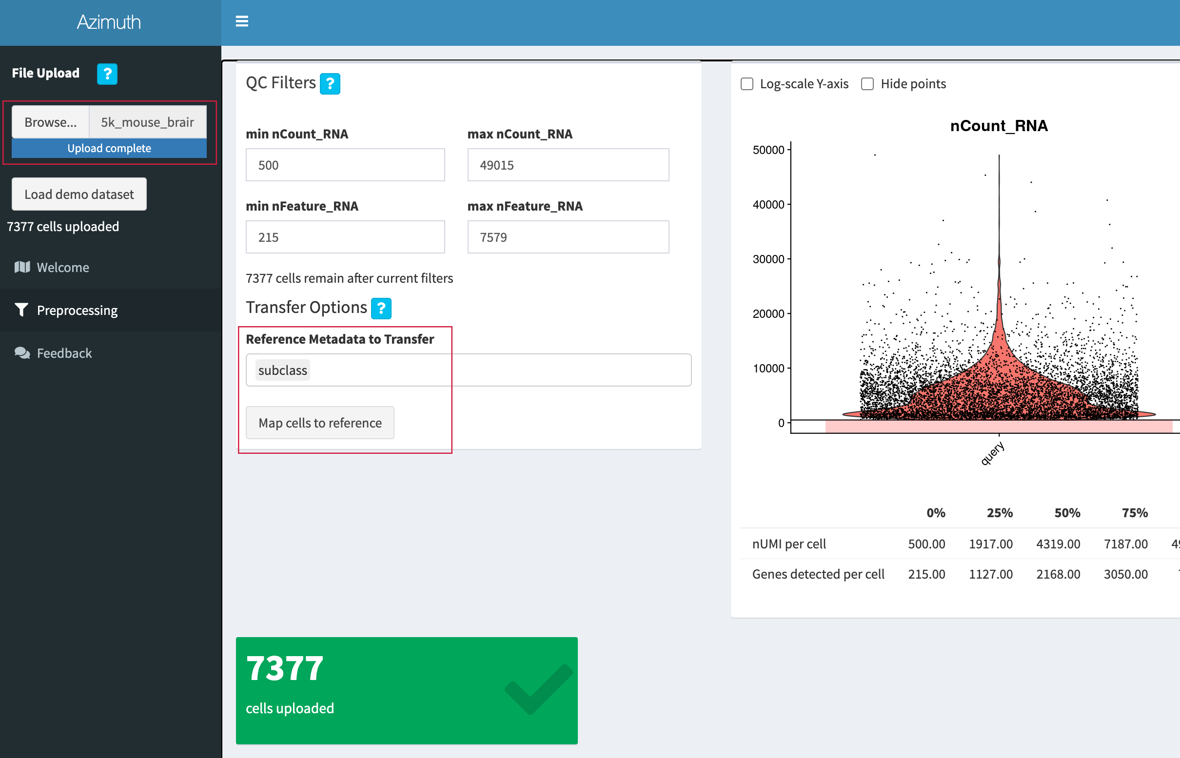
Click "Browse", select the 3' Single Cell Gene Expression
filtered_feature_bc_matrix.h5file (or5k_mouse_brain_CNIK_3pv3_filtered_feature_bc_matrix.h5if downloaded from the public datasets page), and click "Open". -
We will use the "subclass" annotation level. After upload is complete, click "Map cells to reference".

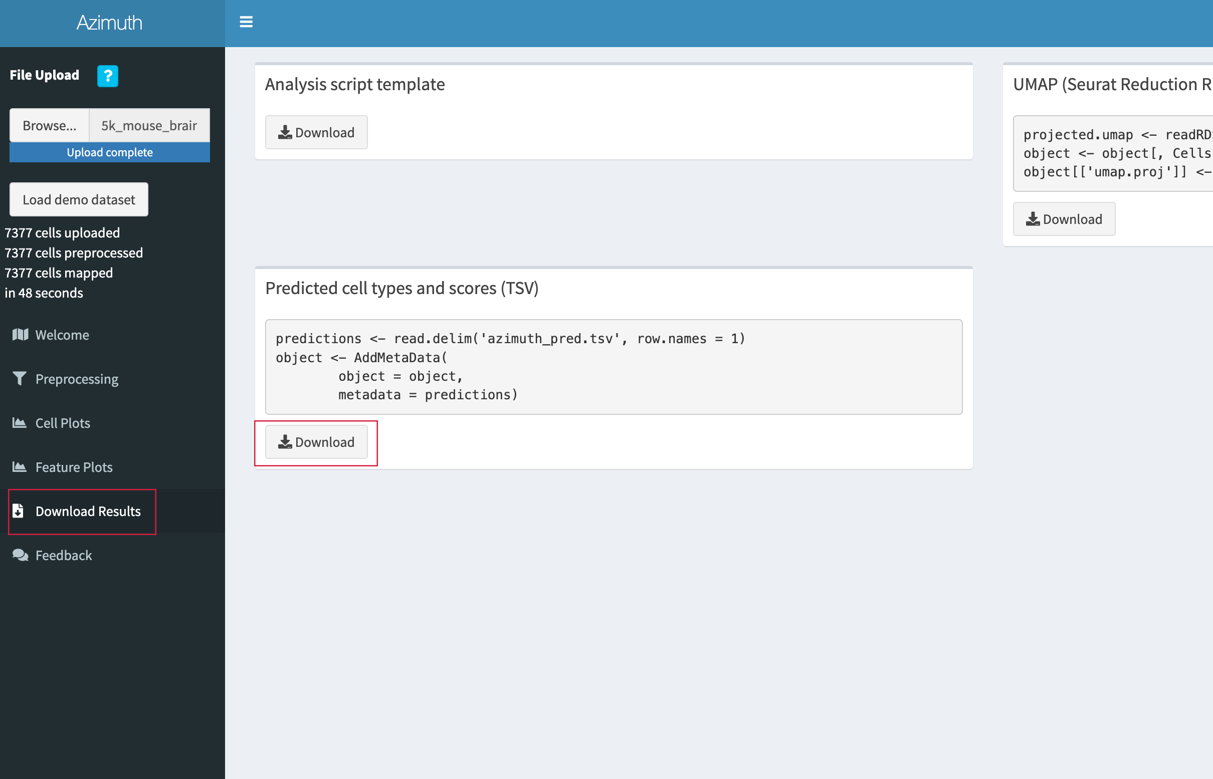
- When annotation is complete, go to the "Download Results" tab and click "Download" under the "Predicted cell types and scores (TSV)" section.

- Save the TSV file in the
adult_mouse_brain_SCdirectory.
Now, read this file into R:
# Load cell types file
cell_types <- read.csv("/path/to/adult_mouse_brain_SC/azimuth_pred.tsv", sep="\t")
head(cell_types)
cell predicted.subclass predicted.subclass.score mapping.score
1 AAACCCAAGGCATCAG-1 Meis2 0.9437153 0.9711163
2 AAACCCAAGGTTCACT-1 L2/3 IT 1.0000000 0.9217411
3 AAACCCACAAAGGCTG-1 L2/3 IT 0.9975360 0.5941127
4 AAACCCACAATGACCT-1 L2/3 IT 1.0000000 0.7366843
5 AAACCCACACGAGGAT-1 Pvalb 0.3933640 0.6632925
6 AAACCCACACTAGTAC-1 L2/3 IT 1.0000000 0.9428686
# Check unique cell types
#unique(cell_types$predicted.subclass)
# Check how many barcodes per cell type annotation
# If needed, update annotation file to meet minimum requirements: spacexr requires at least 25 cells (barcodes) per cell type
table(cell_types$predicted.subclass)
Astro Endo L2/3 IT L5 ET L5 IT L5/6 NP
661 28 1618 128 1088 82
L6 CT L6 IT L6 IT Car3 L6b Lamp5 Meis2
276 574 80 69 84 382
Micro-PVM Oligo OPC Peri Pvalb Sncg
406 1176 149 29 186 13
Sst Sst Chodl Vip VLMC
113 68 49 118
Following spacexr guidance, we modified the cell type names to remove unsupported characters (e.g., "/") and grouped cell types that had fewer than 25 cells (barcodes) per type.
# Remove /
cell_types[cell_types == "L2/3 IT"] <- "L2_3 IT"
cell_types[cell_types == "L5/6 NP"] <- "L5_6 NP"
# Group Sncg (Sncg+ GABAergic neuron) with Sst (Sst+ GABAergic neuron)
cell_types[cell_types == "Sncg"] <- "Sncg_Sst"
cell_types[cell_types == "Sst"] <- "Sncg_Sst"
The Azimuth reference file provides cell-level prediction scores and mapping scores for the cell type annotation for each barcode. Poor annotations can affect deconvolution results (read more about assessing mapping quality here). For this guide, we will keep scores greater than or equal to 0.5.
cell_types_filter <- cell_types[cell_types$predicted.subclass.score >= 0.5 & cell_types$mapping.score >=0.5, ]
Now, format object for spacexr:
#head(cell_types)
# The cell_types object is a dataframe with 4 columns: cell (barcode), predicted subclass (cell type name), predicted subclass score, mapping score
# Set the cell type name and barcode as object names
cell_types <- setNames(cell_types_filter[[2]], cell_types_filter[[1]])
# Convert to factor data type
cell_types <- as.factor(cell_types)
head(cell_types)
AAACCCAAGGCATCAG-1 AAACCCAAGGTTCACT-1 AAACCCACAAAGGCTG-1
Meis2 L2_3 IT L2_3 IT
AAACCCACAATGACCT-1 AAACCCACACTAGTAC-1 AAACCCACAGGTCCCA-1
L2_3 IT L2_3 IT Micro-PVM
head(count_SeuratObject@meta.data)
The nUMI object can be created from the nCount_RNA metadata column in the Seurat Object:
orig.ident nCount_RNA nFeature_RNA
AAACCCAAGGCATCAG-1 SeuratProject 2124 1199
AAACCCAAGGTTCACT-1 SeuratProject 6981 3088
AAACCCACAAAGGCTG-1 SeuratProject 9361 3545
AAACCCACAATGACCT-1 SeuratProject 13741 4284
AAACCCACACGAGGAT-1 SeuratProject 16633 4994
AAACCCACACTAGTAC-1 SeuratProject 8003 3311
# Format for spacexr
sc_umis <- count_SeuratObject@meta.data[,c(1,2)]
# Set object names as nCount_RNA and barcode
sc_umis <- setNames(sc_umis[[2]], rownames(sc_umis))
head(sc_umis)
Now, the UMI counts are formatted per barcode:
AAACCCAAGGCATCAG-1 AAACCCAAGGTTCACT-1 AAACCCACAAAGGCTG-1 AAACCCACAATGACCT-1 AAACCCACACGAGGAT-1 AAACCCACACTAGTAC-1
2124 6981 9361 13741 16633 8003
Finally, use the function below to create a single reference object that contains the count matrix, cell types per barcode, and number of UMIs per barcode.
# Create single cell reference object
SCreference <- Reference(sc_counts, cell_types, sc_umis)
For this demo, we will deconvolve spots with "full" mode, which allows for any number of cell types per spot. Other mode options are "doublet" (one or two cell types per spot) or "multi" (multiple cell types per spot up to a fixed number using a greedy algorithm).
# Optional: spacexr runs faster with more cores, but you may need to adjust system environment settings
Sys.setenv("OPENBLAS_NUM_THREADS"=2)
# Create and run RCTD algorithm
myRCTD <- create.RCTD(VisiumData, SCreference, max_cores = 2)
myRCTD <- run.RCTD(myRCTD, doublet_mode = "full")
The results for "full" mode are stored in the results slot of the myRCTD object.
# Create the output directory in your working directory
resultsdir <- "RCTD_output_plots/" # An output directory for plots, can be any name
dir.create(resultsdir)
# Create variables from the myRCTD object to plot results
barcodes <- colnames(myRCTD@spatialRNA@counts) # list of spatial barcodes
weights <- myRCTD@results$weights # Weights for each cell type per barcode
# Normalize per spot weights so cell type probabilities sum to 1 for each spot
norm_weights <- normalize_weights(weights)
cell_type_names<-colnames(norm_weights) # List of cell types
# dim(norm_weights) # matrix of 2,264 spots and 21 cell types
# For each spot barcode (row), you can see the normalized weight for each cell type (column)
# Look at cell type normalized weights for 2 spots
subset_df <- as.data.frame(t(as.data.frame(norm_weights[1:2,])))
subset_df$celltypes <- rownames(subset_df); rownames(subset_df) <- NULL
subset_df[order(subset_df$`AAACAGAGCGACTCCT-1`, decreasing=T),]
Below are the normalized weights across all 21 cell types from the single cell reference annotation file for two spots, AAACAGAGCGACTCCT-1 and AAACCCGAACGAAATC-1. The five cell types with higher normalized weights for the first spot are:
- "L6 IT" (Layer 6 glutamatergic neuron, intratelencephalon-projecting)
- "Astro" (Astrocyte)
- "Oligo" (Oligodendrocyte)
- "L5 IT" (Layer 5 glutamatergic neuron, intratelencephalon-projecting)
- "Endo" (Endothelial cell)
AAACAGAGCGACTCCT-1 AAACCCGAACGAAATC-1 celltypes
6.882424e-01 3.282160e-01 L6 IT
8.035402e-02 1.250008e-01 Astro
6.694975e-02 1.183004e-01 Oligo
5.234001e-02 9.562916e-05 L5 IT
3.463386e-02 8.976138e-02 Endo
3.231686e-02 9.562916e-05 L2_3 IT
1.274826e-02 2.176886e-02 Micro-PVM
1.186839e-02 1.901338e-02 Peri
9.478824e-03 9.562916e-05 L5_6 NP
8.951182e-03 2.893789e-02 Vip
1.565552e-03 9.562916e-05 VLMC
5.508874e-05 5.950101e-02 Sst Chodl
5.508874e-05 9.562916e-05 L5 ET
5.508874e-05 9.562916e-05 Lamp5
5.508874e-05 9.562916e-05 L6b
5.508874e-05 1.660357e-01 Meis2
5.508874e-05 9.562916e-05 L6 IT Car3
5.508874e-05 2.510426e-02 OPC
5.508874e-05 1.740404e-02 Sncg_Sst
5.508874e-05 9.562916e-05 Pvalb
5.508874e-05 9.562916e-05 L6 CT
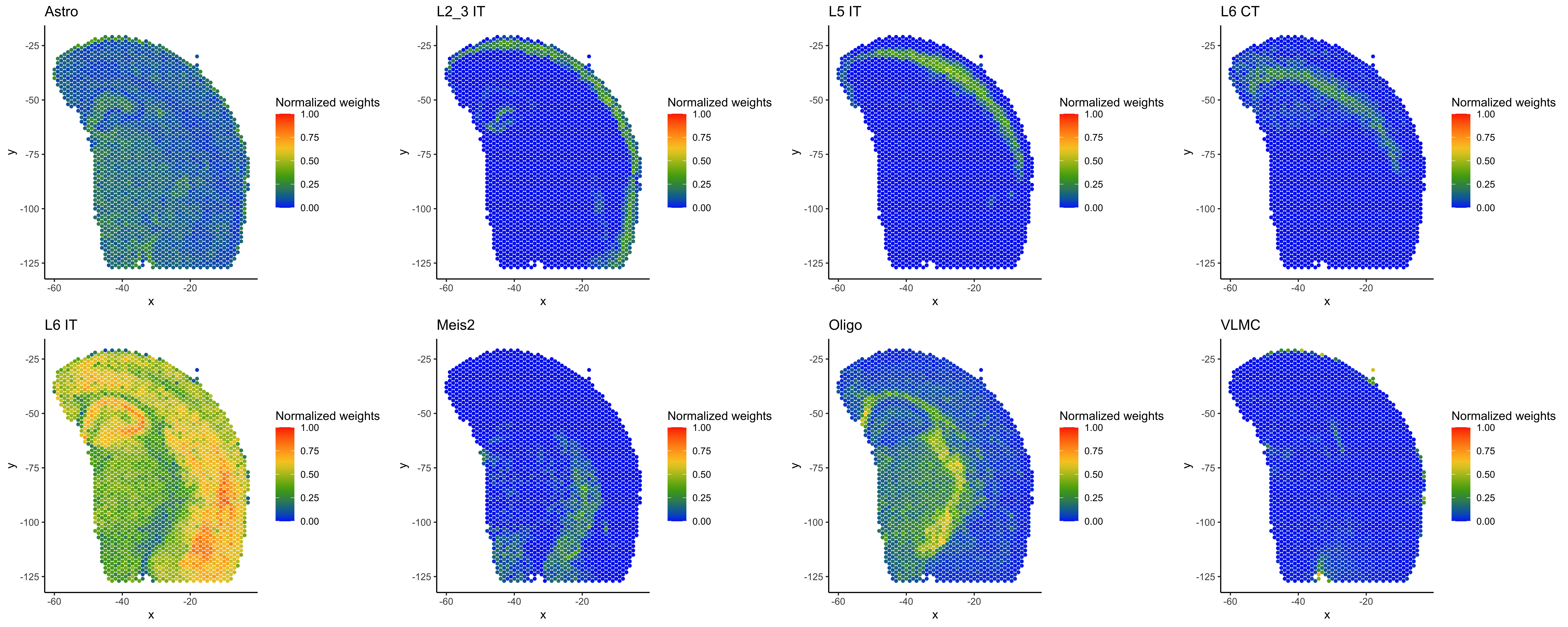
Now, we will plot the normalized weights for the 21 cell types across all spots.
# Plot cell type probabilities (normalized) per spot (red = 1, blue = 0 probability)
# Save each plot as a jpg file
for(i in 1:length(cell_types)){
plot_puck_continuous(myRCTD@spatialRNA, barcodes, norm_weights[,cell_type_names[i]], title =cell_type_names[i], size=1)
ggsave(paste(resultsdir, cell_type_names[i],'_weights.jpg', sep=''), height=5, width=5, units='in', dpi=300)
}
Here are plots showing the normalized weights for eight of the Azimuth mouse motor cortex cell types in different regions of the mouse brain sample:

To interpret the spot deconvolution results, evaluate whether they make sense in light of the sample biology, as well as the cell type reference used for annotation. Refer to the spacexr vignettes and documentation for further guidance on spacexr analyses and outputs.
This spot deconvolution method was used in the Single cell and spatial multiomics identifies Alzheimer’s disease markers Application Note, where the reference data came from multiomic gene expression data. The code from this guide can be used to similarly format inputs from the Application Note's spatial data and multiome gene expression data. Note that the gene expression count data must be specified in this case, as the multiome dataset also contains ATAC data: scdata <- CreateSeuratObject(Counts$`Gene Expression`). In addition, these datasets are much larger than those used in this guide and may require more time and computational resources to complete the analyses.
- Cable et al. Robust decomposition of cell type mixtures in spatial transcriptomics. Nature Biotechnology 40, 517-526 (2022).
- Hao et al. Integrated analysis of multimodal single-cell data. Cell 184, P3573-3587 (2021).
- Li et al. Benchmarking spatial and single-cell transcriptomics integration methods for transcript distribution prediction and cell type deconvolution. Nature Methods 19, 662–670 (2022).
- Yao et al. A transcriptomic and epigenomic cell atlas of the mouse primary motor cortex. Nature 598, 103-110 (2021).
>sessionInfo()
R version 4.2.1 (2022-06-23)
Platform: x86_64-apple-darwin17.0 (64-bit)
Running under: macOS Monterey 12.5
Matrix products: default
LAPACK: /Library/Frameworks/R.framework/Versions/4.2/Resources/lib/libRlapack.dylib
locale:
[1] en_US.UTF-8/en_US.UTF-8/en_US.UTF-8/C/en_US.UTF-8/en_US.UTF-8
attached base packages:
[1] stats graphics grDevices utils datasets methods base
other attached packages:
[1] ggplot2_3.3.6 sp_1.5-0 SeuratObject_4.1.0 Seurat_4.1.1 spacexr_2.0.1
loaded via a namespace (and not attached):
[1] plyr_1.8.7 igraph_1.3.2 lazyeval_0.2.2 splines_4.2.1 listenv_0.8.0
[6] scattermore_0.8 usethis_2.1.6 digest_0.6.29 foreach_1.5.2 htmltools_0.5.2
[11] fansi_1.0.3 magrittr_2.0.3 memoise_2.0.1 tensor_1.5 cluster_2.1.3
[16] doParallel_1.0.17 ROCR_1.0-11 tzdb_0.3.0 remotes_2.4.2 globals_0.15.1
[21] readr_2.1.2 matrixStats_0.62.0 vroom_1.5.7 spatstat.sparse_2.1-1 prettyunits_1.1.1
[26] colorspace_2.0-3 ggrepel_0.9.1 dplyr_1.0.9 callr_3.7.0 crayon_1.5.1
[31] jsonlite_1.8.0 progressr_0.10.1 spatstat.data_2.2-0 survival_3.3-1 zoo_1.8-10
[36] iterators_1.0.14 glue_1.6.2 polyclip_1.10-0 pals_1.7 gtable_0.3.0
[41] leiden_0.4.2 pkgbuild_1.3.1 future.apply_1.9.0 maps_3.4.0 abind_1.4-5
[46] scales_1.2.0 spatstat.random_2.2-0 miniUI_0.1.1.1 Rcpp_1.0.8.3 viridisLite_0.4.0
[51] xtable_1.8-4 reticulate_1.25 spatstat.core_2.4-4 bit_4.0.4 mapproj_1.2.8
[56] htmlwidgets_1.5.4 httr_1.4.3 RColorBrewer_1.1-3 ellipsis_0.3.2 ica_1.0-2
[61] farver_2.1.1 pkgconfig_2.0.3 uwot_0.1.11 deldir_1.0-6 utf8_1.2.2
[66] labeling_0.4.2 tidyselect_1.1.2 rlang_1.0.3 reshape2_1.4.4 later_1.3.0
[71] munsell_0.5.0 tools_4.2.1 cachem_1.0.6 cli_3.3.0 generics_0.1.3
[76] devtools_2.4.3 ggridges_0.5.3 stringr_1.4.0 fastmap_1.1.0 goftest_1.2-3
[81] processx_3.6.1 bit64_4.0.5 fs_1.5.2 fitdistrplus_1.1-8 purrr_0.3.4
[86] RANN_2.6.1 pbapply_1.5-0 future_1.26.1 nlme_3.1-157 mime_0.12
[91] hdf5r_1.3.5 compiler_4.2.1 rstudioapi_0.13 plotly_4.10.0 curl_4.3.2
[96] png_0.1-7 spatstat.utils_2.3-1 tibble_3.1.7 stringi_1.7.6 ps_1.7.1
[101] rgeos_0.5-9 lattice_0.20-45 Matrix_1.4-1 vctrs_0.4.1 pillar_1.7.0
[106] lifecycle_1.0.1 spatstat.geom_2.4-0 lmtest_0.9-40 RcppAnnoy_0.0.19 data.table_1.14.2
[111] cowplot_1.1.1 irlba_2.3.5 httpuv_1.6.5 patchwork_1.1.1 R6_2.5.1
[116] promises_1.2.0.1 KernSmooth_2.23-20 gridExtra_2.3 parallelly_1.32.0 sessioninfo_1.2.2
[121] codetools_0.2-18 dichromat_2.0-0.1 MASS_7.3-57 pkgload_1.3.0 rprojroot_2.0.3
[126] withr_2.5.0 sctransform_0.3.3 mgcv_1.8-40 parallel_4.2.1 hms_1.1.1
[131] quadprog_1.5-8 grid_4.2.1 rpart_4.1.16 tidyr_1.2.0 Rtsne_0.16
[136] shiny_1.7.1